
Statistical Inference - Confidence Interval & Hypothesis Testing
Introduction
Inferential Statistics is the process of examining the observed data (sample) in order to make conclusions about properties/parameter of a Population.
The conclusion of a statistical inference is called a statistical proposition. Some common forms are the following:
- a point estimate (mean)
- an interval estimate (confidence interval)
- rejection of a hypothesis (hypothesis testing)
- clustering or classification of individual data points into groups (Machine Learning techniques, Regression, Classification)
The classic approach for Inferential Statistics requires to make assumptions about the population distribution - which is unknown. If we knew about the Population, there would be no need for Inference!
Hence, using analytical formulas - and making wild assumptions while at it - is not advised. Especially nowadays: with the available processing power and so many readily available programming tools, we can easily make inferences over simulated data distribution.
This post will cover Confidence Interval and Hypothesis Testing.
The code for each method can be found here:
Confidence Interval
Importing necessary libraries and loading the example dataset.
This fictitious dataset contains the average height (in centimeters) of undergrad students, as well as categorical information about age and if they drink coffee.
import pandas as pd
import numpy as np
import matplotlib.pyplot as plt
import seaborn as sns

df_full = pd.read_csv('undergrad_students.csv')
df_full.head(3)
| user_id | age | drinks_coffee | height | |
|---|---|---|---|---|
| 0 | 4509 | <21 | False | 163.93 |
| 1 | 1864 | >=21 | True | 167.19 |
| 2 | 2060 | <21 | False | 181.15 |
We are interested in studying whether the average height for coffee drinkers is the same as for non-coffee drinkers.
Our research question can be rewritten as:
The difference between the average height of Coffee drinkers and No Coffee drinker is equal to zero.
First, let’s create a sample of size 200 from our full dataset. We will call it the “Original Sample”.
Then, we can use the Bootstrapping technique to generate the Sampling Distribution based on the Original Sample.
Finally, we calculate the average height of each group of interest (coffee drinker vs no coffee), compute their difference, and store it in a list called diffs.
We repeat this process 10,000 times so the Central Limit Theory “kicks-in”, resulting in a normally distributed difference in average heights.
Note: this process yields 3 arrays of size 10,000: average height of coffee drinkers; average height of those who do not drink coffee, and the difference in means.
df_sample = df_full.sample(200)

# instantiate empty list
diffs = []

# Bootstraping 10,000 times
for _ in range(10_000):
    boot_sample = df_sample.sample(len(df_sample), replace=True)
    avg_height_coffee = boot_sample.query('drinks_coffee == True').height.mean()
    avg_height_not_coffee = boot_sample.query('drinks_coffee == False').height.mean()
    diffs.append(avg_height_coffee - avg_height_not_coffee)

print(f'Sampling Distribution Mean: {np.mean(diffs):.3f} cm')
print(f'Sampling Distribution Std: {np.std(diffs):.3f} cm')
Sampling Distribution Mean: 3.394 cm
Sampling Distribution Standard Deviation: 1.193 cm
# Actual difference in average height, based on the original sample
height_coffee = df_sample.query('drinks_coffee == True').height
height_no_coffee = df_sample.query('drinks_coffee == False').height

actual_avg_height_difference = height_coffee.mean() - height_no_coffee.mean()
print(f'Original Sample average height difference: {actual_avg_height_difference:.3f} cm')
Original Sample average height difference: 3.390 cm
Checking the difference between the average height of both groups, we can see the mean of our Sampling Distribution (3.394 cm) closely approximates the actual average height difference observed in the original sample (3.390 cm).
Calculating Lower and Upper Bounds
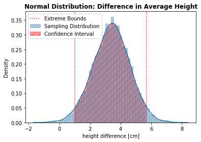
Lastly, let’s find the lower and upper bounds of the interval containing the correct parameter with a confidence level of 95%:
alpha = 5.0
lower, upper = np.percentile(diffs, alpha/2) , np.percentile(diffs, 100 - alpha/2)
print(f'Confidence Interval: [{lower:.2f}, {upper:.2f}]')
Confidence Interval: [1.01, 5.70]
# Plotting
ax = sns.distplot(diffs, hist_kws={'edgecolor':'gray'}, label='Sampling Distribution')
...
CI_width = upper - lower
print(f'Average Height Difference: {np.mean(diffs):.2f} cm')
print(f'Margin of error: {CI_width/2:.2f} cm')
Average Height Difference: 3.39 cm
Margin of error: 2.34 cm
Interpretation
Since the Confidence Interval does not contain (overlap) zero, there is evidence that suggests there is indeed a difference in the population height of those sub-groups. As a matter of fact, there is a substantial difference since the lower bound is far from zero.
We have evidence to support that, on average, coffee drinkers are taller than those who do not drink coffee. We can infer, with 95% confidence, the average height difference is 3.4 cm with a margin of error of 2.3 cm.
- bigger sample size narrower Confidence Interval width
- Margin of Error: Confidence Interval width / 2
Hypothesis Testing
Another form of Inferential Statistics, helps to make better and data-informed decisions. This technique is vastly implemented in research, academia, and A/B testing.
- Translate research question into 2 clearly defined and competing hypothesis:
- Null
- Alternative
- Collect data (Experiment Design: ideal sample size, how long to conduct, consistency among control and experiment groups etc.) to evaluate both hypothesis.
Also:
- We assume the Null, , to be true before even collecting the data (prior belief)
- always holds some sign of equality sign ( )
- The Alternative, , is what we would like to prove to be true
- always holds the opposite sign of the Null ( )
Setting Up Hypothesis
It is usually easier to start defining the Alternative Hypothesis and what sign it should hold: is it bigger? Is it different? Is it smaller?
Then, the Null assumes the opposite sign (with some sort of equality).
- Example 1: The new assembly technique is better than the existing one
- Measurement: proportion of defective product,
- Example 2: The average height of coffee drinkers is different than non-coffee drinkers
- Measurement: average height,
- Example 3: The new website design is better than the existing one
- Measurement: subscription rate,
Significance Testing
There are two alternative ways of computing the statistical significance of a parameter inferred from a data set, in terms of a test statistic: One-tailed test and a Two-tailed test.
- One-tailed test: Used when we are interested in testing if the Alternative is better (lesser or greater than, depending on the metric)
- Two-tailed test: Used when we are interested in just testing if the Alternative is different
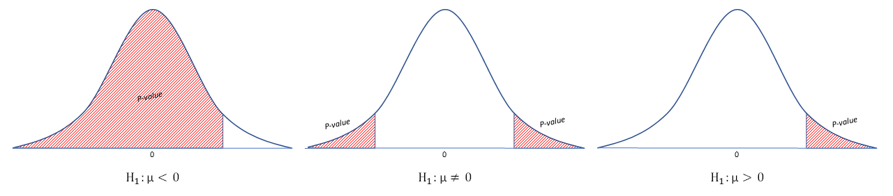
In the image above we see an example of the result for each possible setup of the Alternative Hypotheses, being: lesser; different; and greater.
Where:
-
The Bell curve represents the distribution of all possible values, assuming the Null Hypotheses to be true/correct. The blue curve is drawn from the Null, with the mean value as the closest value to the Null (in this case, 0).
-
The hashed area in red is the p-value, representing all values that actually support the Alternative Hypotheses (“equal or more extreme than”). Note how the hashed area
does not necessarilystarts from the closest value to the Null (in this case, 0). -
The graphic seen above is the famous Probability Density Function (PDF). The area under this curve represents the probability, which cumulative sum varies between 0 and 1.
Assuming the Null to be true/correct, we draw the blue bell-shaped curve. P-value is the area under this curve (probability) for values that are equal or more extreme than data supporting the Alternative.
p-value: probability of seeing data that actually supports the Alternative, assuming the Null to be true/correct.
Interpreting the p-value
This is a very hot topic, involving hyped claims and the dismissal of possibly crucial effects, much due to the fact of using “significant results only” () as a publishing criteria on peer-reviewed journals.
We never “accept” a Hypothesis, since there is always the chance of it being wrong - even if very small.
Instead, we either Reject or Fail to Reject the Null:
- Small p-value: we Reject the Null. Rather, the statistics is likely to have come from a different distribution.
- Big p-value: we Fail to Reject the Null. It is indeed likely the observed statistic came from the distribution assuming the Null to be true.
But what is small and big ?
The p-value is compared against (alpha), the rate of False Positives we are willing to accept.
Note: the concept of and False Positives will be further explained in the Decision Errors section.
Danger of Multiple Tests
As mentioned before, there is always the chance of randomly finding data supporting the Alternative. Even if the p-value is quite small!
For the usually accepted Significance Level of 5% (), it basically means that if we perform the same experiment 20 times (), we expect that one of them will result in a False Positive… and we are okay with it!
Whenever replicating the same experiment, or conducting multiple tests (i.e. A/B testing using more than one metric), we need to watch out for compounding of Type I error (error propagation)!
Enter the Correction Methods for multiple tests:
- Bonferroni:
- The Type I error rate should be the desired , divided by the number of tests, .
- Example: if replicating the same experiment 20 times, each experiment corrected would be = 0.0025 (that means, 0.25% instead of the initial 5%).
- As illustrated in the example above, this method is very conservative. While it does minimize the rate of False Positives (making the findings more meaningful), it also fails to recognize actual significant differences. Which increases the amount of Type II error (False Negatives), leading to a test with low Power.
- Holm-Bonferroni: recommended approach
- Less conservative, this adaptation from the Bonferroni method presents a better trade-off between Type I and II errors.
- It consist of a simple but tricky to explain algorithm. See this Wikipedia for detailed explanation.
- I personally created a Python function to implement this method. It receives a list of the identification of the test/metric/experiment, and another with the respective p-value of each individual test/experiment. The output is a list of all tests that have evidence to Reject the Null; and another one with the remaining, where we Fail to Reject the Null. The code can be found in the A/B Testing post.
Pitfalls
- When interpreting statistical significance results, we assume the sample is truly representative of the Population of interest.
- It is important to watch out for Response Bias, when only a specific segment of the population is captured in the sample.
- Example: people against a bill (or project) are more likely to attend a Public Hearing to manifest their opinion than those in favor.
- With large enough sample size, hypothesis testing leads to even the smallest differences being considered as statistically significant.
- Hence, it is important to be aware of Practical Significance as well, taking into consideration extraneous factors such as: cost, time etc.
- Example: a small improvement in the manufacturing process - even if statistically significant - might not be worth the cost, time, and/or effort to implement it.
Decision Errors (False Positives & False Negatives)
Whenever making decisions without knowing the correct answer, we can face 4 different outcomes:
- Correct:
- True Positives
- True Negatives
- Wrong:
- False Positives
- False Negatives
Enters the Confusion Matrix:
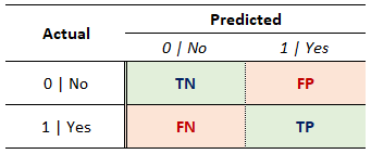
- Type I error (False Positive):
- Reject the Null when it is actually true
- The probability of committing a Type I error is represented by (also know as Significance Level)
- Not committing it () is know as Confidence Level
- Type II error (False Negative):
- Fail to reject the Null when it is indeed false
- Probability of committing a Type II error is represented by
- Not committing it () is known as the Power of the test
Common values used in practice are:
- Significance Level () = 5%
- Test Power ()= 80%
Differentiating between Type I (False Positive) and Type II (False Negative) errors can be confusing… until you see this image:

Hypothesis Testing in Practice
Importing necessary libraries and loading the example dataset.
This fictitious dataset contains the average height (in centimeters) of undergrad students, as well as categorical information about age and if they drink coffee.
import pandas as pd
import numpy as np
import matplotlib.pyplot as plt
import seaborn as sns

df_full = pd.read_csv('undergrad_students.csv')
df_full.head(3)
| user_id | age | drinks_coffee | height | |
|---|---|---|---|---|
| 0 | 4509 | <21 | False | 163.93 |
| 1 | 1864 | >=21 | True | 167.19 |
| 2 | 2060 | <21 | False | 181.15 |
Example 1
We are interested in studying the average height of undergrad students.
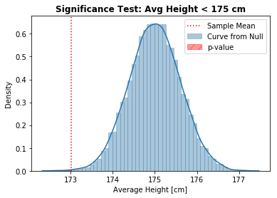
Research Question 1: the average height of people who drink coffee is greater than 175 cm
- cm
- cm
# Take initial sample of size 200 from the dataset
df_sample = df_full.sample(200)

# Calculate average height of coffee drinkers
sample_mean = df_sample.query('drinks_coffee == True').height.mean()
print(f'Sample Mean: {sample_mean:.2f} cm')
Sample Mean: 173.02 cm
# Generate Sampling Distribution of average height of coffee drinkers
sampling = []

for _ in range(10_000):
    boot_sample = df_sample.sample(len(df_sample), replace=True)
    avg_height_coffee = boot_sample.query('drinks_coffee == True').height.mean()
    sampling.append(avg_height_coffee)

print(f'Sampling Distribution Std: {np.std(sampling):.2f} cm')
Sampling Distribution Standard Deviation: 0.61 cm
# Assuming the Null is True, generate curve of possible values
null_mean = 175 # closest value possible to the Null

null_curve = np.random.normal(null_mean, np.std(sampling), 10_000)
Note: Since the Alternative is “greater than” (), the shaded area goes from the Sample Mean to the right .
# Plotting
ax = sns.distplot(null_curve, hist_kws={'edgecolor':'gray'}, label='Curve from Null');
...

# calculate p-value
pvalue = (null_curve > sample_mean).mean()
print(f'p-value = {pvalue:.3f}')
p-value = 0.999
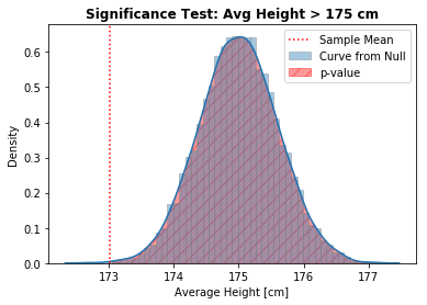
Interpretation: With such a high p-value (0.94), we Fail to Reject the Null Hypotheses. Suggesting the average height of coffee drinkers is equal or lesser than 175 cm.
It looks like the statistic of interest (sample mean) does come from a Normal Distribution centered around 175 (closest value to the Null) and with the Standard Deviation from the Sampling Distribution.
Example 2
Research Question 2: the average height of people who drink coffee is lesser than 175 cm
- cm
- cm
Note: Since the Alternative is “lesser than” (), the shaded area goes from the Sample Mean to the left.
# Plotting
ax = sns.distplot(null_curve, hist_kws={'edgecolor':'gray'}, label='Curve from Null');
...

# calculate p-value
pvalue = (null_curve < sample_mean).mean()
print(f'p-value = {pvalue:.3f}')
p-value = 0.001
Interpretation: Since the p-value (0.001) is lesser than (0.05), we have evidence to Reject the Null Hypotheses, suggesting - with 95% of confidence - that the average height of coffee drinkers is indeed smaller than 175 cm.
The statistic of interest (sample mean) is likely to have come from a different distribution.
Example 3
Research Question 3: the average height of people who drink coffee is different than 175 cm
- cm
- cm
Note: Since the Alternative is “different than” (), the shaded area goes from the most extreme lower and upper bounds, to the outside.
print(f'Sample Mean: {sample_mean:.2f} cm')
print(f'Null Mean: {null_mean:.2f} cm')
Sample Mean: 173.02 cm
Null Mean: 175.00 cm (closest value to the Null)
Since the Sample Mean is smaller than the Null:
- Lower Bound: Sample Mean
- Upper bound:
lower = sample_mean
upper = null_mean + (null_mean - sample_mean)

# Plotting
ax = sns.distplot(null_curve, hist_kws={'edgecolor':'gray'}, label='Curve from Null');
...

# Calculate p-value
pvalue = (null_curve < lower).mean() + (null_curve > upper).mean()
print(f'p-value = {pvalue:.3f}')
p-value = 0.001
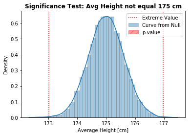
Interpretation: Since the p-value (0.001) is lesser than (0.05), we have evidence to Reject the Null Hypotheses, suggesting - with 95% of confidence - that the average height of coffee drinkers is indeed different than 175 cm.
As a sanity check, this result supports the conclusion from the previous test, where we had evidence suggesting the average height of coffee drinkers to be lesser than 175 cm.
Main Takeaways
Note how Hypothesis Testing results does not provide a definitive answer. We merely Reject or Fail to Reject the Null Hypothesis. Hence, translating the research question into the hypothesis to be tested is the critical step for this Inference method.
Also, Confidence Interval and Hypothesis Testing only allow to make observations over a Population Parameter. In order to make decisions on the individual level, one should use Machine Learning methods such as Regression and Classification (to be covered in the next post!).
As always, constructive feedback is appreciated. Feel free to leave any questions/suggestions in the comments section below!