Linear Regression Part 1 - Linear Models

Introduction

Linear Regression is the linear approach to modeling the relationship between a quantitative response ($y$) and one or more explanatory variables ($X$); also known as Response and Features, respectively.

This post focuses on Simple and Multiple Linear Model, also covering Flexible Linear Model (higher order and interaction terms).

The code can be found in this Notebook.

Let’s load the data and necessary libraries. The toy dataset used in this example contain information on house prices and its characteristics, such as Neighborhood, square footage, # of bedrooms and bathrooms.

import pandas as pd
import numpy as np
import seaborn as sns
import matplotlib.pyplot as plt
%matplotlib inline

df = pd.read_csv('house_prices.csv')
df.drop(columns='house_id', inplace=True)
df.head(3)

	neighborhood	area	bedrooms	bathrooms	style	price
0	B	1188	3	2	ranch	598291
1	B	3512	5	3	victorian	1744259
2	B	1134	3	2	ranch	571669

Correlation Coefficient, $R$

Measure of strength and direction of linear relationship between a pair of variables. Also know as Pearson’s correlation coefficient.

• Value varies between [-1, 1], representing negative and positive linear relationship
• Strength:
  • $0 \leq R < 0.3$: Weak correlation
  • $0.3 \leq R < 0.7$: Moderate correlation
  • $R \geq 0.7$: Strong correlation

df.corr().style.background_gradient(cmap='Wistia')

	area	bedrooms	bathrooms	price
area	1	0.901623	0.891481	0.823454
bedrooms	0.901623	1	0.972768	0.743435
bathrooms	0.891481	0.972768	1	0.735851
price	0.823454	0.743435	0.735851	1

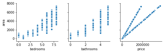
A scatter plot between two variables is a good way to visually inspect correlation:

sns.pairplot(data=df,y_vars='area', x_vars=['bedrooms', 'bathrooms','price']);

Example of Pair Plot between quantitative variables

Ordinary Least Squares Algorithm

The main algorithm used to find the line that best fit the data. It minimizes the sum of squared vertical distance between the fitted line and the actual points.

$$\sum^n_{i=1}(y_i - \hat y_i)^2$$

Basically, it tries to minimize the error.

Example of a Simple Linear Model

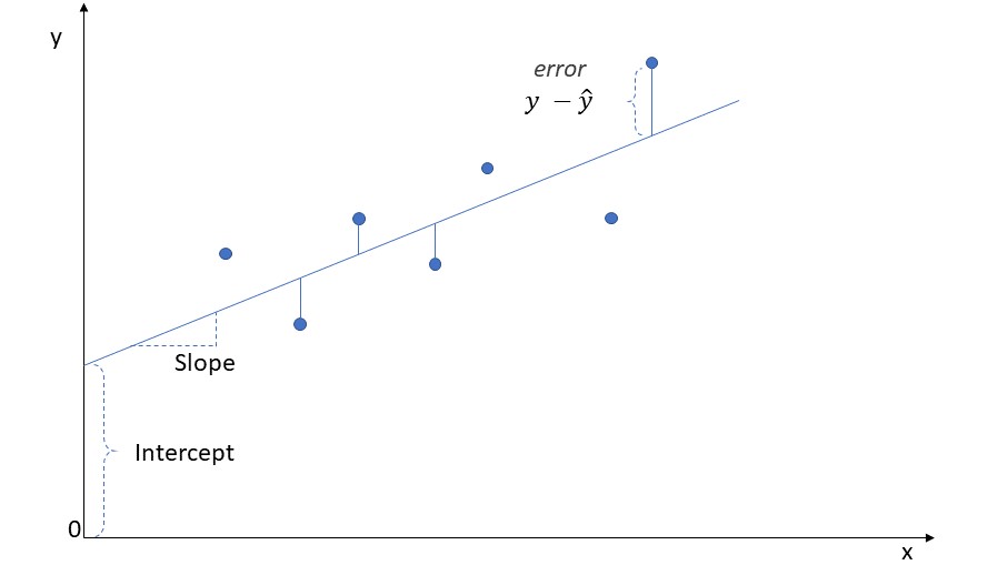
A Simple Linear Regression Model can be written as:

$$\hat y = b_0 + b_1.x_1 $$

Where,

• $\hat y$: predicted response
• $b_0$: intercept. Height of the fitted line when $x=0$. That is, no influence from explanatory variables
• $b_1$: coefficient. The slope of the fitted line. Represents the weight of the explanatory variable

The Statsmodels package is a good way to obtain linear models, providing pretty and informative results, such as intercept, coefficients, p-value, and R-squared.

Note 1: Statsmodels requires us to manually create an intercept = 1 so the algorithm can use it. Otherwise, the intercept is fixed at 0.

Note2: Different than Scikit-Learn, Statsmodels requires the response variable as the first parameter.

import statsmodels.api as sm
df['intercept'] = 1
# Note how Statsmodels uses the order (y, X)
model = sm.OLS(df.price, df[['intercept', 'area']])
results = model.fit()
results.summary2()

Model:	OLS	Adj. R-squared:	0.678
Dependent Variable:	price	AIC:	169038.2643
Date:	2019-04-03 16:30	BIC:	169051.6726
No. Observations:	6028	Log-Likelihood:	-84517.
Df Model:	1	F-statistic:	1.269e+04
Df Residuals:	6026	Prob (F-statistic):	0.00
R-squared:	0.678	Scale:	8.8297e+10

	Coef.	Std.Err.	t	P>|t|	[0.025	0.975]
intercept	9587.8878	7637.4788	1.2554	0.2094	-5384.3028	24560.0784
area	348.4664	3.0930	112.6619	0.0000	342.4029	354.5298

Interpretation

In this simple example, we are tying to predict house prices as a function of their area (in square feet).

• intercept: it means the starting point for every house is 9,588 price unit

• coefficient: being a quantitative variable, it means that for every 1 area unit increase, we expect 345.5 increase in the price unit, on top of the intercept.

• p-value: represents if a specific variable is significant in the model. If p-value > $\alpha$, then we can discard that variable from the model without significantly impacting its predictive power.

  It always tests the following Hypothesis:

$$H_0: \beta =0 $$ $$H_1: \beta \neq 0$$

• R-squared: it is a metric of model performance (coefficient of determination). Represents the amount of observations that can be “explained” by the model. In this case, 0.678 or 67.8%.
  • It is calculated as the square of the Correlation Coefficient, hence its value varies between [0, 1].

Note: R-squared is a metric only capturing linear relationship. Better and more robust forms of model evaluation are covered in Part 3 of this Linear Regression series, such as accuracy, precision, and recall.

Multiple Linear Regression

But it is also possible to incorporate more than just one explanatory variable in our linear model:

$$\hat y = b_0 + b_1.x_1 + b_2.x_2 + ... + b_n.x_n$$

Let’s fit a linear model using all quantitative variables available:

df['intercept'] = 1
# Note how Statsmodels uses the order (y, X)
model = sm.OLS(df.price, df[['intercept', 'area','bedrooms','bathrooms']])
results = model.fit()
results.summary2()

Model:	OLS	Adj. R-squared:	0.678
Dependent Variable:	price	AIC:	169041.9009
Date:	2019-04-03 16:30	BIC:	169068.7176
No. Observations:	6028	Log-Likelihood:	-84517.
Df Model:	3	F-statistic:	4230.
Df Residuals:	6024	Prob (F-statistic):	0.00
R-squared:	0.678	Scale:	8.8321e+10

	Coef.	Std.Err.	t	P>|t|	[0.025	0.975]
intercept	10072.1070	10361.2322	0.9721	0.3310	-10239.6160	30383.8301
area	345.9110	7.2272	47.8627	0.0000	331.7432	360.0788
bedrooms	-2925.8063	10255.2414	-0.2853	0.7754	-23029.7495	17178.1369
bathrooms	7345.3917	14268.9227	0.5148	0.6067	-20626.8031	35317.5865

Interpretation

Since the p-value of bedrooms and bathrooms is greater than $\alpha$ (0.05), it means these variables are not significant in the model. Which explains why the R-squared didn’t improve after adding more features.

As a matter of fact, it is all about multicollinearity: as it happens, there is an intrinsic correlation between these explanatory variables.

You would expect a house with more bedrooms and bathrooms to have a higher square footage!

It is also the reason behind the unexpected flipped sign for the bedrooms coefficient.

Just as well, you would expect a house with more bedrooms to become more and more expensive; not cheaper!

This and other potential modeling problems will be covered in more details later, in Part 2. But basically, in situations like this, we would remove the correlated features from our model, retaining only the “most important one”.

The “most important one” can be understood as:

• A specific variable we have particular interest in understanding/capturing
• A more granular variable, allowing for a better representation of the characteristics our model is trying to capture
• A variable easier to obtain

In this case, let’s discard the others quantitative variables and use only area as predictor in the model:

df['intercept'] = 1
# Note how Statsmodels uses the order (y, X)
model = sm.OLS(df.price, df[['intercept', 'area']])
results = model.fit()
results.summary2()

Model:	OLS	Adj. R-squared:	0.678
Dependent Variable:	price	AIC:	169038.2643
Date:	2019-04-03 16:30	BIC:	169051.6726
No. Observations:	6028	Log-Likelihood:	-84517.
Df Model:	1	F-statistic:	1.269e+04
Df Residuals:	6026	Prob (F-statistic):	0.00
R-squared:	0.678	Scale:	8.8297e+10

	Coef.	Std.Err.	t	P>|t|	[0.025	0.975]
intercept	9587.8878	7637.4788	1.2554	0.2094	-5384.3028	24560.0784
area	348.4664	3.0930	112.6619	0.0000	342.4029	354.5298

Interpretation

The adjusted R-squared remained at 0.678, indicating we didn’t lose much by dropping bedrooms and bathrooms from our model.

So, considering the quantitative variables available, we should only use area.

But what about the categorical variables?

Working with Categorical Data

So far we have only worked with quantitative variables in our examples. But it is also possible to work with Categorical data, such as Neighborhood or Style.

We can use Hot-One encoding, creating new dummy variables receiving value of 1 if the category is true, or 0 otherwise.

We can easily implement this by using the pandas.get_dummies function.

Note: we use the pd.get_dummies function inside the df.join, in order to add the created columns to the already existing dataframe.

df = df.join(pd.get_dummies(df.neighborhood, prefix='neighb'))
df = df.join(pd.get_dummies(df['style'], prefix='style'))
df.head(2)

	neighborhood	area	bedrooms	bathrooms	style	price	intercept	neighb_A	neighb_B	neighb_C	style_lodge	style_ranch	style_victorian
0	B	1188	3	2	ranch	598291	1	0	1	0	0	1	0
1	B	3512	5	3	victorian	1744259	1	0	1	0	0	0	1

But before we can incorporate the categorical data in the model, it is necessary to make sure the selected features $X$ are Full Rank. That is, all explanatory variables are linearly independent.

If a dummy variable holds the value 1, it specifies the value for the categorical variable. But we can just as easily identify it if all other dummy variables are 0.

Therefore, all we need to do is leave one of the dummy variables out of the model - for each group of categorical variable. This “left out” variable will be the baseline for comparison among the others from the same category.

Let’s use only Neighborhood (A, B, C) and Style (Victorian, Lodge, Ranch) in our model:

# neighborhood Baseline = A
# style Baseline = Victorian
feature_list = ['intercept', 'neighb_B', 'neighb_C', 'style_lodge','style_ranch']

# Note how Statsmodels uses the order (y, X)
model = sm.OLS(df.price, df[feature_list])
results = model.fit()
results.summary2()

Model:	OLS	Adj. R-squared:	0.584
Dependent Variable:	price	AIC:	170590.6058
Date:	2019-04-03 16:30	BIC:	170624.1267
No. Observations:	6028	Log-Likelihood:	-85290.
Df Model:	4	F-statistic:	2113.
Df Residuals:	6023	Prob (F-statistic):	0.00
R-squared:	0.584	Scale:	1.1417e+11

	Coef.	Std.Err.	t	P>|t|	[0.025	0.975]
intercept	836696.6000	8960.8404	93.3726	0.0000	819130.1455	854263.0546
neighb_B	524695.6439	10388.4835	50.5074	0.0000	504330.4978	545060.7899
neighb_C	-6685.7296	11272.2342	-0.5931	0.5531	-28783.3433	15411.8841
style_lodge	-737284.1846	11446.1540	-64.4133	0.0000	-759722.7434	-714845.6259
style_ranch	-473375.7836	10072.6387	-46.9962	0.0000	-493121.7607	-453629.8065

Interpretation

Using both categorical data at the same time, our model resulted in an R-squared of 0.584. Which is less than obtained before with quantitative data… but it still means there is some explanatory power to these categorical variables.

All variables seem to be significant, with p-value < $\alpha$. Except for Neighborhood C.

This means neighb_C is not statistically significant in comparison to the baseline, neighb_A.

To interpret the significance between a dummy and the other variables, we look at the confidence interval (given by [0.025 and 0.975]): if they do not overlap, then it is considered significant. In this case, neighb_C is significant to the model, just not when compared to the baseline… suggesting that Neighborhood A shares the same characteristics of Neighborhood C.

• intercept: represents the impact of the Baselines. In this case, we expect a Victorian house located in Neighborhood A to cost 836,696 price unit.

• Coefficients: since we only have dummy variables, they are interpreted against their own category baseline

  • neighb_B: we predict a house in Neighborhood B to cost 524,695 more than in Neighborhood A (baseline). For a Victorian house, it would cost 836,696 + 524,695 = 1,361,391 price unit.
  • neighb_C: since its p-value > $\alpha$, it is not significant compared to the baseline - so we ignore the interpretation of this coefficient
  • style_lodge: we predict a Lodge house to cost 737,284 less than a Victorian (baseline). In Neighborhood A, it would cost 836,696 - 737,284 = 99,412 price unit
  • style_ranch: we predict a Ranch to cost 473,375 less than a Victorian (baseline). In Neighborhood A, it would cost 836,696 - 473,375 = 363,321 price unit

Putting it all together

Now that we covered how to work with and interpret quantitative and categorical variables, it is time to put it all together:

Note: we leave Neighborhood C out of the model, since our previous regression - using only categorical variables - showed it to be insignificant.

In this case, Neighborhood A is no longer the Baseline and needs to be explicitly added to the model:

# style Baseline = Victorian
feature_list = ['intercept', 'area', 'neighb_A', 'neighb_B', 'style_lodge', 'style_ranch']

# Note how Statsmodels uses the order (y, X)
model = sm.OLS(df.price, df[feature_list])
results = model.fit()
results.summary2()

Model:	OLS	Adj. R-squared:	0.919
Dependent Variable:	price	AIC:	160707.1908
Date:	2019-04-03 16:30	BIC:	160747.4158
No. Observations:	6028	Log-Likelihood:	-80348.
Df Model:	5	F-statistic:	1.372e+04
Df Residuals:	6022	Prob (F-statistic):	0.00
R-squared:	0.919	Scale:	2.2153e+10

	Coef.	Std.Err.	t	P>|t|	[0.025	0.975]
intercept	-204570.6449	7699.7035	-26.5686	0.0000	-219664.8204	-189476.4695
area	348.7375	2.2047	158.1766	0.0000	344.4155	353.0596
neighb_A	-194.2464	4965.4594	-0.0391	0.9688	-9928.3245	9539.8317
neighb_B	524266.5778	4687.4845	111.8439	0.0000	515077.4301	533455.7254
style_lodge	6262.7365	6893.2931	0.9085	0.3636	-7250.5858	19776.0588
style_ranch	4288.0333	5367.0317	0.7990	0.4243	-6233.2702	14809.3368

Looks like Neighborhood A is not significant to the model. Let’s remove it and interpret the results again:

# style Baseline = Victorian
feature_list = ['intercept', 'area', 'neighb_B', 'style_lodge', 'style_ranch']

# Note how Statsmodels uses the order (y, X)
model = sm.OLS(df.price, df[feature_list])
results = model.fit()
results.summary2()

Model:	OLS	Adj. R-squared:	0.919
Dependent Variable:	price	AIC:	160705.1923
Date:	2019-04-03 16:30	BIC:	160738.7132
No. Observations:	6028	Log-Likelihood:	-80348.
Df Model:	4	F-statistic:	1.715e+04
Df Residuals:	6023	Prob (F-statistic):	0.00
R-squared:	0.919	Scale:	2.2149e+10

	Coef.	Std.Err.	t	P>|t|	[0.025	0.975]
intercept	-204669.1638	7275.5954	-28.1309	0.0000	-218931.9350	-190406.3926
area	348.7368	2.2045	158.1954	0.0000	344.4152	353.0583
neighb_B	524367.7695	3908.8100	134.1502	0.0000	516705.1029	532030.4361
style_lodge	6259.1344	6892.1067	0.9082	0.3638	-7251.8617	19770.1304
style_ranch	4286.9410	5366.5142	0.7988	0.4244	-6233.3477	14807.2296

Looking at the high p-values of style_lodge and style_ranch, they do not seem to be significant in our model.

Let’s regress our model again, removing style_lodge.

Note: since we are removing Lodge, Victorian style no longer is the baseline, hence we have to explicitly add it to the model

feature_list = ['intercept', 'area', 'neighb_B', 'style_victorian', 'style_ranch']

# Note how Statsmodels uses the order (y, X)
model = sm.OLS(df.price, df[feature_list])
results = model.fit()
results.summary2()

Model:	OLS	Adj. R-squared:	0.919
Dependent Variable:	price	AIC:	160705.1923
Date:	2019-04-03 16:30	BIC:	160738.7132
No. Observations:	6028	Log-Likelihood:	-80348.
Df Model:	4	F-statistic:	1.715e+04
Df Residuals:	6023	Prob (F-statistic):	0.00
R-squared:	0.919	Scale:	2.2149e+10

	Coef.	Std.Err.	t	P>|t|	[0.025	0.975]
intercept	-198410.0294	4886.8434	-40.6009	0.0000	-207989.9917	-188830.0672
area	348.7368	2.2045	158.1954	0.0000	344.4152	353.0583
neighb_B	524367.7695	3908.8100	134.1502	0.0000	516705.1029	532030.4361
style_victorian	-6259.1344	6892.1067	-0.9082	0.3638	-19770.1304	7251.8617
style_ranch	-1972.1934	5756.6924	-0.3426	0.7319	-13257.3710	9312.9843

Once again, neither Victorian nor Ranch proved to be significant in the model.

Let’s remove style_ranch:

feature_list = ['intercept', 'area', 'neighb_B', 'style_victorian']

# Note how Statsmodels uses the order (y, X)
model = sm.OLS(df.price, df[feature_list])
results = model.fit()
results.summary2()

Model:	OLS	Adj. R-squared:	0.919
Dependent Variable:	price	AIC:	160703.3098
Date:	2019-04-03 16:30	BIC:	160730.1265
No. Observations:	6028	Log-Likelihood:	-80348.
Df Model:	3	F-statistic:	2.287e+04
Df Residuals:	6024	Prob (F-statistic):	0.00
R-squared:	0.919	Scale:	2.2146e+10

	Coef.	Std.Err.	t	P>|t|	[0.025	0.975]
intercept	-199292.0351	4153.3840	-47.9831	0.0000	-207434.1541	-191149.9162
area	348.5163	2.1083	165.3055	0.0000	344.3833	352.6494
neighb_B	524359.1981	3908.4435	134.1606	0.0000	516697.2501	532021.1461
style_victorian	-4716.5525	5217.5622	-0.9040	0.3660	-14944.8416	5511.7367

Looks like the house style is not significant at all in our model.

Let’s also remove Style Victorian from our explanatory variables:

feature_list = ['intercept', 'area', 'neighb_B']

# Note how Statsmodels uses the order (y, X)
model = sm.OLS(df.price, df[feature_list])
results = model.fit()
results.summary2()

Model:	OLS	Adj. R-squared:	0.919
Dependent Variable:	price	AIC:	160702.1274
Date:	2019-04-03 16:30	BIC:	160722.2399
No. Observations:	6028	Log-Likelihood:	-80348.
Df Model:	2	F-statistic:	3.430e+04
Df Residuals:	6025	Prob (F-statistic):	0.00
R-squared:	0.919	Scale:	2.2146e+10

	Coef.	Std.Err.	t	P>|t|	[0.025	0.975]
intercept	-198881.7929	4128.4536	-48.1734	0.0000	-206975.0391	-190788.5467
area	347.2235	1.5490	224.1543	0.0000	344.1868	350.2602
neighb_B	524377.5839	3908.3313	134.1692	0.0000	516715.8561	532039.3117

Interpretation

Finally, all features are significant (p-value < $\alpha$).

Interestingly, the adjusted R-squared never changed through the process of eliminating insignificant explanatory variables, meaning these final ones are indeed the most important ones for predicting house price.

Basically, it means that for every 1 area unit increase, we expect an increase of 347 price unit. If a house is situated in Neighborhood B, we expect it to cost, on average, 524,377 more than in Neighborhoods A or C.

Even though the intercept has a negative value, this equation resulted in the best predicting performance so far (adjusted R-squared of 0.919). One can argue that every house - even the smallest one - still have area greater than 0. For houses in Neighborhood A and C with square footage greater than 580, we start to predict positive values for price.

Flexible Linear Models

The linear model is also capable of incorporating non-linear relationships between the explanatory variables and the response, such as: Higher Order and Interaction.

Higher Order

Whenever there is a clear curve-like pattern between the pair plot of an explanatory variable $x_i$ and the response $y$.

• the higher order should always be the amount of peaks + 1. For example, in a U shaped pair plot, there is 1 peak, hence the feature should be of order 2:

$$x_i^2$$

• whenever using higher order terms in the model, it is also necessary to include the lower order terms. In this example of order 2, we would have the following terms:

$$\hat y = b_0 + b_1.x_1 + b_2.x_1^2$$

Interaction

Whenever the relationship between a feature ($x_1$) and the response ($y$) change according to another feature ($x_2$)

• the need for an interaction term can be visually investigated by adding the hue parameter (color) to the typical pair plot. If the relationship of $x_1$ and $y$ have different slopes based on $x_2$, then we should add the interaction term:

$$x_1.x_2$$

• Similarly to higher order, if implemented in the model, it is also necessary to add the “lower” terms, so the model would look like this:

$$\hat y = b_0 + b_1.x_1 + b_2.x_2 + b_3.x_1.x_2$$

Downside

But there is a caveat: while the prediction power of the linear model improves by adding flexibility (higher order and interaction), it loses the ease of interpretation of the coefficients.

It is no longer straightforward - as seen in the previous models - to interpret the impact of quantitative or categorical variables. Any change in the explanatory variable would be reflected in the simple term, $b_1.x_1$ as well as the higher order one, $b_2.x_1^2$.

Enter the trade-off of linear models: flexible terms might improve model performance, but at the cost of interpretability.

If you are interested in understanding the impact of each variable over the response, it is recommended to avoid using flexible terms.

… and if you are only interested in making accurate predictions, than Linear Models would not be your best bet anyway!

sns.pairplot(data=df, y_vars='price', x_vars=['area', 'bedrooms','bathrooms']);

Pair plot between the Response and quantitative Explanatory Variables

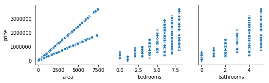
The relationship between the features and the response does not present any curves. Hence, there is no base to implement a higher order term in the model.

# Pair plot by Neighborhood
sns.lmplot(x='area', y='price', data=df, hue='neighborhood', size=4,
           markers=['o','x','+'], legend_out=False, aspect=1.5)
plt.title('Pair plot of Price and Area by Neighborhood');

Pair plot of Price and Area, by Neighborhood

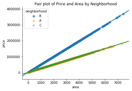
It is clear to see in the image above that the relationship between area and price does vary based on the neighborhood. Which suggests we should add the interaction term.

In this particular case, Neighborhood A and C have the exact same behavior. Therefore, we only need to verify whether the house is located in Neighborhood B or not (using the dummy variable, neighb_B).

# Creating interaction term to be incorporated in the model
df['area_neighb'] = df.area * df.neighb_B

df['intercept'] = 1
features_list = ['intercept', 'area','neighb_B','area_neighb']
model = sm.OLS(df.price, df[features_list])
result = model.fit()
result.summary2()

Model:	OLS	Adj. R-squared:	1.000
Dependent Variable:	price	AIC:	71986.6799
Date:	2019-04-03 16:30	BIC:	72013.4966
No. Observations:	6028	Log-Likelihood:	-35989.
Df Model:	3	F-statistic:	6.131e+10
Df Residuals:	6024	Prob (F-statistic):	0.00
R-squared:	1.000	Scale:	8986.8

	Coef.	Std.Err.	t	P>|t|	[0.025	0.975]
intercept	12198.0608	3.1492	3873.3747	0.0000	12191.8872	12204.2343
area	248.1610	0.0013	194094.9191	0.0000	248.1585	248.1635
neighb_B	132.5642	4.9709	26.6682	0.0000	122.8195	142.3089
area_neighb	245.0016	0.0020	121848.3887	0.0000	244.9976	245.0055

Interpretation

Our best model performance, with an impressive adjusted R-squared of 100%. All variables are significant and their signs match the expected direction (positive).

Although the interpretation is not as easy as before, we can still try to make some sense out of it because this is a special case of interaction, involving a binary variable.

• intercept: we expect all houses to have the initial price of 12,198 price unit.
• Coefficients:
  • for houses in Neighborhood A and C, we expect the price to increase by 248 price unit for every additional area unit. So, the average price of a house of 120 sqft situated in Neighborhood A or C is: $12,198 + 248*120 = 41,958$
  • for houses in Neighborhood B, we expect the price to increase by 493 (248 + 245) price unit for every additional area unit. There would also be an additional 132 price unit on top of the intercept, independent of the area. So the average price of a house of 120 sqft located in Neighborhood B is: $12,198 + (132) + 120*(248 + 245) = 71,490$

Conclusion

In this post we reviewed the basics of Linear Regression, covering how to model and interpret the results of Simple and Multiple Linear Models - working with quantitative as well as categorical variables.

We also covered Flexible Linear Models, when to implement them, and the intrinsic trade-off between flexibility and interpretability.

In the next post (Part 2), we will focus on some of the potential modeling problems regarding the basic assumptions required for Regression models, covering some strategies on how to identify and address them. Namely, 1) Linearity, 2) Correlated Errors, 3) Non-constant Variance of Errors, 4) Outliers and Leverage Points, and 5) Multicollinearity.

---

As always, constructive feedback is appreciated. Feel free to leave any questions/suggestions in the comments section below!