Statistical Inference - Concepts Review

Introduction

This post will cover the fundamental concepts of the Law of Large Numbers and the Central Limit Theory, both of which are essential for practical statistical inference (Confidence Interval and Hypothesis Testing - to be covered in another post). Importing necessary libraries and loading the example dataset.

The full code can be found in this notebook.

The example dataset contains the average height (in centimeters) of undergrad students, as well as categorical information about age and if they drink coffee.

	user_id	age	drinks_coffee	height
0	4509	<21	False	163.93
1	1864	>=21	True	167.19
2	2060	<21	False	181.15

Law of Large Numbers

Bigger sample size will result in a statistic that more closely represents the Population parameter.

This can be demonstrated by comparing the Population Parameter - average height ($\mu$) - against the Sample Statistic - average height $\bar X$.

Let’s assume:

• the full dataset, df_full, represents the Population.
• different samples, randomly selected from the full dataset, using specific sample sizes.

Population Avg Height: 171.698 cm
Population Size: 2,974

# Different sizes, from 3 to 2974, with increments of 10
sizes = range(3,len(df_full),10)

# List Comprehension: Random sampling, for all different sample sizes
avg_heights = [df_full.sample(size).height.mean() for size in sizes]

# Plotting
plt.plot(sizes, population_mean - avg_heights)
plt.axhline(0, color='r', linestyle=':', label='Population Mean')
...

Law of Large Numbers explained

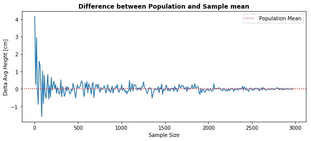
As stated on the Law of Large Numbers, we verify that larger samples yield an estimated statistic closer to the “actual value” (population parameter). That is, the difference between the Population and Sample average height converges to zero.

Central Limit Theory

With a large enough sample size, the sampling distribution of specific statistics will be normally distributed around the mean value.

This applies to some, but not all statistics: mean, proportion, difference in means, difference in proportions.

Similar to what we have done before, this can be demonstrated by generating sampling distributions based on different sample sizes.

But first, what is a “sampling distribution” and how can we obtain one?

• Sampling Distribution: shows the frequency of every possible result a statistic can take in every possible sample from a population.

• Bootstrapping: Estimate the Sampling Distribution of any statistic by constructing a number of resamples with replacement of the observed dataset (and of equal size to the observed dataset).

Let’s see an example: Take a small sample of size 50 from the dataset.
Generate sampling distribution of average height, considering the following amount of repetition (resample):

• 100
• 1,000
• 10,000
• 80,000

# From the original dataset, take a small sample of size 50
df_sample_50 = df_full.sample(50)

# Generate Sampling Distribution with 100 resamples
resampling_100 = np.random.choice(df_sample_50.height, (100, 50)).mean(axis=1)
...

# Plotting it all together, with same x and y axis
sns.distplot(resampling_100, ax=axes[0,0], hist_kws={'edgecolor':'gray'})
axes[0,0].set_title('Resamples: 100')
...

Central Limit Theory explained

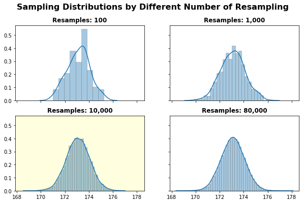
As stated by the Central Limit Theory, we can verify that a larger amount of resampling will indeed lead to a normal distribution, centered around the mean value. As a matter of fact, the highlighted plot - with 10,000 repetitions - seems to result in a “good enough” normal.

Law of Large Numbers + Central Limit Theory

Now, it is only natural to combine the best of both concepts, having a normal distribution based on a sample “big enough” to result in an accurate estimator for the Population Parameter.

Let’s investigate this by replicating the 10,000 resampling based on initial samples of different sizes:

• 50
• 100
• 200
• 1,000

# From the original dataset, take different sample sizes
df_sample_50 = df_full.sample(50)
df_sample_100 = df_full.sample(100)
...

# Bootstrap for each sample, replicating 10,000 times
bootstrap_50 = np.random.choice(df_sample_50.height, (10_000, 50)).mean(axis=1)
...

# Plotting it all together, with same x and y axis
sns.distplot(bootstrap_50, ax=axes[0,0], hist_kws={'edgecolor':'gray'})
axes[0,0].axvline(population_mean, color='r', label='Population Mean')
axes[0,0].axvline(bootstrap_50.mean(), color='k', label='Sample Mean')
...

Combining both concepts

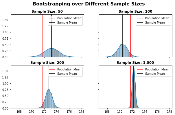
As expected, with 10,000 resamples the Central Limit Theory “kicks-in”, resulting in Normally Distributed sampling distributions.

Also, due to the Law of Large Numbers, larger sample sizes results in a more accurate estimate of the Population Parameter. We can see that, as the sample size increases:

• the difference between the Population and Sample means decrease
• the Confidence Interval width decrease

$\implies$ Meaning we become more confident of estimating the correct value.

Main Takeaway

By combining both concepts, we can obtain a pretty accurate estimate of the population parameter - even based on a small sample size, such as 200 observations. As long as we resample it 10,000 times.

Hence, these are the reference values arbitrarily specified for our practical approach of inferential statistics, both for Confidence Interval and Hypothesis Testing, covered in another post.

---

As always, constructive feedback is appreciated. Feel free to leave any questions/suggestions in the comments section below!